Central Limit Theorem (cont.)

A more technical exploration of the CLT and how it fits into the rest of statistics

Premise

In a previous post I wrote a short story attempting to illustrate a statistical concept, the Central Limit Theorem. I certainly overlooked some things about it, so here I want to dive a little more into the technical details, using the help of code to explain why this result is so cool and useful.

To begin we need to talk about a few statistical concepts. Let’s start with the idea of a population.

Say you want to learn something about a group of things—for instance, the average number of books (the thing we want to know) owned by people who live in New York City (the group). The “population” here is everyone in NYC, without exclusion. (In the ideal, statistics is the epitome of inclusivity.)

To find the average, you would need to ask every New Yorker (minus the non-city folks) how many books they own, then do a simple calculation.

The average is a number that summarizes something about the population under consideration. It’s one way of getting at the expected number of books owned by a random New Yorker. Because you are counting every person in NYC, the result is the “true” average. There is no uncertainty regarding the calculation. It is a capital-T Truth of the world. (At least if you assume the population is fixed and unchanging, which we will do so here: no new books are allowed to be purchased or obtained. I know, it hurts—sorry!) Statisticians call this the population mean.

Reality

Sadly the above scenario is an idealization. It is simply not feasible—if not downright impossible—to account for every person living in NYC. We could get book counts for some of them, even many of them, but our average would fall short of the population mean, the capital-T truth.

But how short? Might there be a way to get reasonably close? What is reasonably close? Enter: Statistics.

Friend of few, bane of all (hey there’s a truth), statistics is what you get when you are not God. If you were you wouldn’t need it. You wouldn’t need to do it. You would just know that the average number of books owned by people who live in NYC is [redacted: the population mean]. Philberto enters the scene.

Philberto: Hey now, you can’t just know the average like that. That’s not your role. You, human, must suffer through the pesky statistical procedures your kind has invented to discover it. Effort only does the truth reward, so effortful effort you must give...

Philberto poofs into a cloud of smoke, sails away in a drift of wind as quickly as he arrived.

What was that about? Buckle up I guess… we’re stuck with statistics.

Statistics

If you want to know the average number of books owned by every New Yorker, a pragmatic approach would be to ask who you already know.

Okay, so you do that. You surveyed your ten close friends (are you an outlier?) and compute an average: 40.2 books. Would this be a good guess for the number of books a random person in NYC owns?

No for several reasons, but they all touch on the same issue: your friends do not represent every New Yorker. They are your friends after all. They’ve been subject to social, cultural, and economic selection processes that would bias any conclusion you make about the whole of NYC.

You accept this and expand your survey to include neighbors and people you don’t know so well but are familiar with. After knocking on every door around the block, your new average is: 15.7 books.

What a drop! Are some New Yorkers really not as sophisticated (or intellectually performative) as you initially thought? The prospect saddens you. But at least your estimate feels more plausible. You’ve included more people, and the uncertainty has shrunk.

You consider continuing—expanding the survey further—but you realize you are tired and would actually like to read the books you own. This is more fun than counting them, and you abandon your statistical quest. Philberto looks down in shame.

The Computation of Poetics

Let’s summarize what we’ve done so far.

We attempted to infer a population quantity (the true average) given only a fraction of the population—a sample. In reality, all we ever have are samples: parts of the whole we’re interested in, which we use to learn something about the world. I want to focus now on an important result that builds from this process.

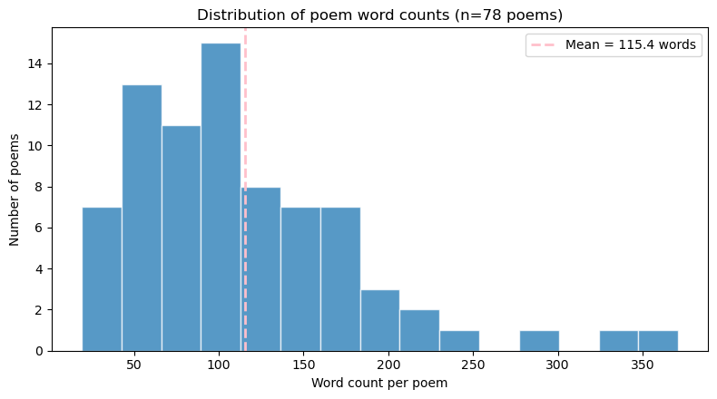
Let’s say there exists only 78 poems in the universe. This is my universe, at least if I consider the universe to be the number of poems sitting in one of my Google Docs. These 78 poems constitute a population, and I want to know something about it: what is the average word count across every poem in this universe?

Since I have access to the whole population, calculating the true average is straightforward. I can count the words in each poem and compute the mean. This turns out to be 115.4 words, as depicted in the histogram below. Most poems sit between 50 and 150 words, with a handful of longer outliers.

Now imagine Philberto strips me of my godly omniscience. He takes away my knowledge of the true average—and even the list of poems themselves. The only thing he leaves me with is the ability to access 20 poems at random. I can use these 20 poems to calculate an average, but it’s clear that it won’t equal the true average. I’m no longer accounting for every poem in the universe, and so my estimate is uncertain.

Still, it turns out we can get at the true average through the following process:

1. Select 20 poems at random

2. Count the total number of words in each

3. Compute the average

4. Repeat steps 1–3 many times, producing a collection of averages

5. Compute the average of those averages

This final quantity—the average of the sample averages—ends up extremely close to the true population mean. In the limit of infinitely many repetitions, it equals it exactly. Importantly, this repetition does not create the population mean; it merely reveals that the sampling process is already centered on it.

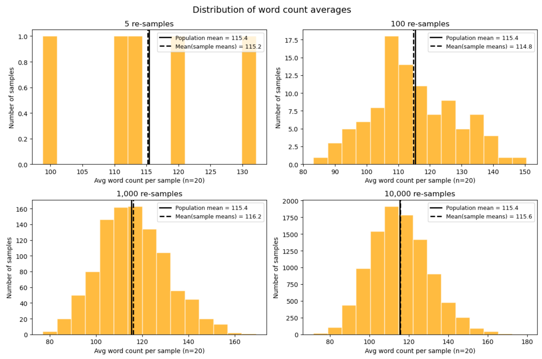
What we see is that, as the number of repetitions increases, two things happen:

1. The mean of the sample means stabilizes around the population mean.

2. The shape of the sampling distribution becomes clearer and smoother.

This bell-shaped curve—the hallmark of the Central Limit Theorem (CLT)—does not appear because we repeat the process more often. It appears because each average pools many independent observations. Repetition simply allows us to see that shape more clearly. From variability and randomness, a certain kind of order emerges.

The Poetics of Computation

It is rarely the case that we can draw from the same population many times. That is, we often only have one sample of data to work with. So how does the CLT help us? In short: it enables us to reason about uncertainty.

Pretend again I only have access to 20 random poems from my poetic universe. This means I can compute exactly one average. This average would be my best guess at the true mean word count. How off is it as an estimate?

I can’t answer that question directly—I can’t know the true mean because I do not have access to the entire population. But I can ask something slightly different:

If the true mean were some value, how likely would it be that I observed the average I did?

This reframe is at the heart of statistical reasoning. We do not learn the truth by repetition (resamples) of the world itself. Instead we imagine repetition in order to test our beliefs about a single observation. What makes this “move” possible is the Central Limit Theorem.

It tells us how our estimate would fluctuate if we could repeat the process under the same conditions. That imagined distribution gives us a way to measure uncertainty—to attach margins of error, to build confidence intervals, and to decide when an observation is surprising enough to warrant doubt. We assume what the truth is, temporarily, and gauge what we see relative to that assumption.

***

Let’s make this concrete. Say the average word count of the 20 random poems I have access to is 111.3 words. Now, if I assume the true average word count is 100 words, how likely is it that I would observe my average, 111.3 words? To answer this, I need more than my one observed average. I need a way to imagine what other averages might have looked like, had I drawn a different random set of 20 poems.

This is where the Central Limit Theorem enters the picture. It tells me that if I were to repeat this sampling process many times—each time selecting 20 poems at random and computing their average—the averages would themselves form a distribution. This distribution of averages would be centered on the (assumed) true average and would have a predictable spread. It is approximately normal (bell-shaped), even when the underlying population is not.

Given this—that we know the exact shape of the distribution—we don’t actually need to perform the repeated sampling. We can simply imagine a normal distribution centered on the assumption that the true word count is 100 words (and that we are randomly sampling 20 poems—this is what determines the spread) and compute the probability of observing the average we got (111.3 words). Let’s see this pictorially.

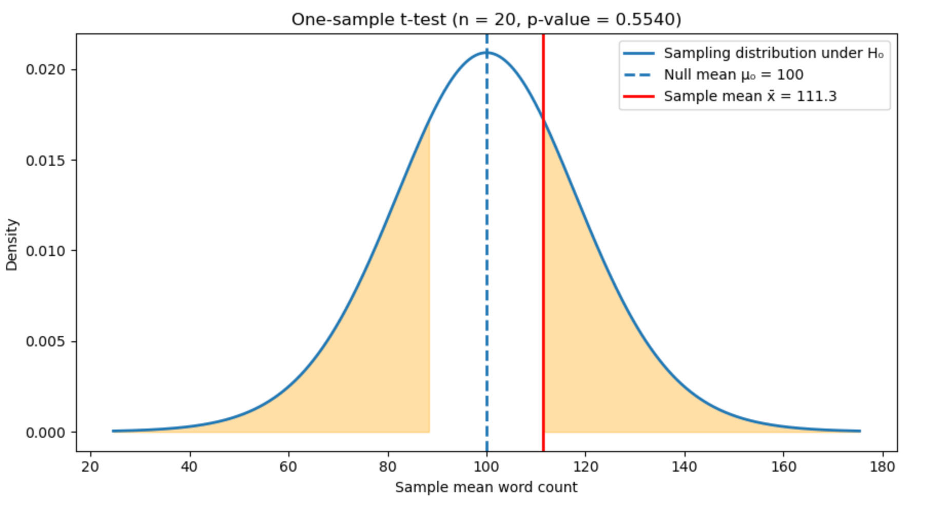
The curve in the figure does not describe the poems themselves, but a hypothetical world in which the true mean word count is 100. The blue dashed line marks this assumption, the mean we assume to be true. What I actually observed is marked by the red solid line. It’s not far off from the assumed mean. How to quantify this?

The orange regions represent averages that would be at least as extreme as what I observed in this hypothetical world. The probability of landing in these regions is what statisticians call the “p-value.” In this case the regions are large, meaning my observation is not at all surprising if the true average word count were really 100 words. More exactly, if we assume the true average word count is 100, about 55.4% of random samples of 20 poems would produce an average that differs from 100 by at least as much as the one I observed.

***
Researchers typically set a threshold beyond which they determine a result to be surprising using the approach outlined above (known as Null Hypothesis Significance Testing, or NHST). Usually this threshold is 0.05: if the p-value is less than 0.05 the “null hypothesis”—the assumption that the true average word count is 100—is rejected. My p-value here is 0.554, so I do not reject the null.

Note that I bolded the assumption. This is because I don’t actually know what the true average is, nor can I discovering it with Null Hypothesis Significance Testing (NHST). The p-value is merely the probability of observing our data under a specific set of assumptions, not the likelihood that any given hypothesis is true. It’s a statement about what we observed if a particular model of the world were true.

Whether or not this model of the world is true is a separate question, one that is more difficult to get at, even if we care about it more. Put another way: the true average word count in my document of poems either is or isn’t 100 words. Determining the likelihood of either case requires a different approach, one that is focused on the plausibility of various hypotheses rather than the surprise of seeing what we see if a given hypothesis (the null) were true.

***

It’s worth stepping back now to name exactly the role the Central Limit Theorem has been playing in all of this.

The CLT doesn’t tell us what the true average word count is. It doesn’t allow us to discover it directly, nor does it guarantee that our estimates are correct. What it does instead is more subtle and powerful. It tells us something about what an average is.

When we compute an average from a random sample, it does not stand alone on its own. It belongs to a family of possible averages that could have been observed under the same conditions (the same sampling procedure, the same population, etc). This family is described by the CLT. It tells us that, for sufficiently large samples, averages behave in a regular, predictable way: they gather around the true mean, and their variability shrinks.

Uncertainty hence takes a shape, a pattern, which enables us to reason about it. We would otherwise have no way of saying whether an observed average is surprising, ordinary, or extreme. A single observed average becomes interpretable under the CLT, not because we repeat the world, but because we can imagine how it would behave under repetition. That imagined repetition is not a claim about reality. It is a tool for reasoning under ignorance.

Perhaps put more poetically, what survives aggregation when individual observations are messy, strange, and bewildering is revealed by the CLT. It tells us that while the world may be wild, our summaries of it are not entirely ungoverned.

***

Whether or not the average word count in a collection of poems tells us anything interesting about it is another story. In fact I do not have to be Philberto to say that something is wrong if we can conclude something meaningful about a poem based on word count alone.

Still, there’s something poetic about the search. And word count does count in the sense that poems, some at least, aim for sparsity. That a poem might deviate from the average—from the norm—might be a reflection of the times, a call being answered to uproot culture.

Who is out there writing the next Iliad, the modern Divine Comedy? We might find out if we ask enough poets.